My previous post acted as an introduction to arithmetic coding, using the 1MB Sorting Problem as a case study. I ended that post with the question of how to work with fractional values having millions of significant binary digits.

The answer is that we don’t have to. Let’s work with 32-bit fixed-point math instead, and see how far that gets us.

A 32-bit fixed-point number can represent fractions in the interval [0, 1) using 32 bits of precision. In other words, it can encode the first 32 bits of any binary fraction. To define such a fixed-point number, we simply take a regular 32-bit unsigned integer, and imagine it as the top of a fraction over 2³².

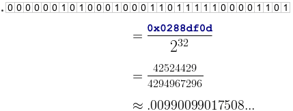
As you can see, 0x0288df0d represents a fixed-point number approximately equal to D, which in the previous post, we estimated as the probability of encountering a delta value of 0 in one of our sorted sequences. It’s actually not such a bad approximation, either: The error is within 0.00000023%.

If you recall the way we partitioned the real number line in the previous post, 0x0288df0d would represent the boundary between the first and second partitions. In a similar way, we can compute the boundaries around all of the first 63 partitions

and compile them into a lookup table:

static const u32 LUTsize = 64;
const u32 LUT[LUTsize] = {
    0x00000000, 0x0288df0d, 0x050b5170, 0x07876772,
    0x09fd3131, 0x0c6cbea6, 0x0ed61f9d, 0x113963bd,
    0x13969a84, 0x15edd348, 0x183f1d3b, 0x1a8a8766,
    0x1cd020ad, 0x1f0ff7cc, 0x214a1b5e, 0x237e99d4,
    0x25ad817f, 0x27d6e088, 0x29fac4f7, 0x2c193cad,
    0x2e32556d, 0x30461cd1, 0x3254a056, 0x345ded53,
    0x366210ff, 0x3861186f, 0x3a5b1096, 0x3c500649,
    0x3e40063a, 0x402b1cfa, 0x421156fd, 0x43f2c095,
    0x45cf65f7, 0x47a75337, 0x497a944b, 0x4b49350b,
    0x4d134131, 0x4ed8c45a, 0x5099ca03, 0x52565d8e,
    0x540e8a41, 0x55c25b43, 0x5771dba1, 0x591d1649,
    0x5ac41611, 0x5c66e5b1, 0x5e058fc6, 0x5fa01ed4,
    0x61369d41, 0x62c9155d, 0x6457915a, 0x65e21b51,
    0x6768bd44, 0x68eb8119, 0x6a6a709d, 0x6be59584,
    0x6d5cf96c, 0x6ed0a5d9, 0x7040a435, 0x71acfdd4,
    0x7315bbf3, 0x747ae7b7, 0x75dc8a2c, 0x773aac4a
};

You’ll recognize this lookup table as the same one found in the source code listing.

The Encoder

We begin the encoding process by setting up a writeInterval structure having two fixed-point members: lo and range. Initially, lo = 0 and range = 0xffffffff.

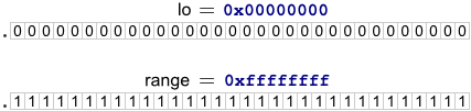
This represents an interval along the real number line. Obviously, range is slightly less than 1.0, so we aren’t quite taking advantage of the full number line, but it’s very close, and it fits inside 32 bits.

Next, we’re going to subdivide this interval. Subdividing is a straightforward matter of linear interpolation. Given a fixed-point value x, we locate the corresponding point within our interval by performing a lerp:

To implement this formula using 32-bit fixed-point math, we must cast to 64 bits before multiplying, then right-shift the result by 32.

u32 lerp(u64 x)        { return lo + (u32) ((range * x) >> 32); }

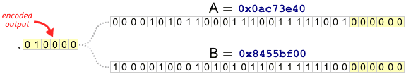
Now, suppose we wish to encode an initial delta value of 29. First, we need to find the boundaries of the partition which corresponds to 29. To find them, we consult LUT[29] and LUT[30] in our lookup table, lerp those values within the writeInterval, and assign the results to A and B. In this case, we end up with A = 0x402b1cf9 and B = 0x421156fc. Since this is the very first partition along the number line, we immediately know that our final encoded binary fraction will lie somewhere within the interval [A, B).

You’ll notice that A and B share the same first 6 bits. We can go ahead and write those 6 bits to the output stream, because they’ll never change, no matter what the final encoded binary fraction ends up being. So let’s write them, then shift both A and B to the left by 6 bits each.

We can now think of A and B as trailing digits on the encoded output. At this point, we’ve written the binary digits we’re sure about, and A and B represent the digits we’re not sure about yet. We need to continue subdividing to drill deeper and gain more certainty about subsequent digits.

Before handling the next delta value in the input sequence, we set up a new writeInterval, setting lo to A, and range to B - A. We then process the next delta value in the same way we did the first, interpolating new A and B values within the new writeInterval. Once again, we output all of the most significant bits which A and B agree on, shifting those values to compensate. We repeat these steps until the entire input sequence is exhausted, at which point we encode a dummy value somewhere within in the final interval (I chose 32), then flush the contents of A to the bit stream.

It turns out that shifting the values of A and B to the left is critical: By shifting them, we maximize the resulting value of range, so there’s always enough numerical precision to subdivide further. This trick lets us get away with using 32-bit fixed point math at every step during the encoding process.

Breaking Up Large Deltas

The lookup table we defined, LUT, contains only 64 entries. Obviously, we can’t use it to look up partition boundaries for delta values greater than 62. We could, perhaps, extend it to hold all 100000001 possible boundary values, but if we did, our fixed-point representation would quickly run out of numerical precision. Check the partitioned number line again: the partition for delta value 10000 is already very close to 1.0. In fact, it would require more than 143 fractional binary digits to represent the boundaries of this partition; way more than 32. And the partitions to the right of that would require even more.

We need a better way. If you do the math, the partition boundaries are actually described by the following function:

And lucky for us, this function satisfies a useful relation:

This relation is basically just another lerp like the one we saw earlier. It tells us that if we want to encode any delta value that is greater than or equal to 63, we can simply reduce the delta value by 63 and encode it within the subinterval [LUT(63), 1) instead.

If the delta value is very large, we simply repeat the reduction step until we have a delta value less than 63. You’ll notice this technique bears some similarity to the Golomb encoding strategy I described earlier, except that it doesn’t encode bits explicitly; only implicitly, as the result of continuous subdivision of the writeInterval.

    void pushDelta(u32 delta)
    {
        while (delta >= LUTsize - 1)
        {
            encode(LUTsize - 1); // Use the [LUT(63), 1) subinterval
            delta -= LUTsize - 1;
        }
        encode(delta);
    }

The Decoder

As you’d expect, the decoder reverses the arithmetic encoding process, also using 32-bit fixed-point math. It begins by setting up a readInterval structure with lo = 0 and range = 0xffffffff, then reads the first 32 binary digits of the encoded bit stream into a fixed-point value readSeq.

That’s all the information the decoder needs to correctly determine the first delta value. It finds this delta value by performing a binary search through the lookup table, lerping every LUT entry through the readInterval until it identifies the partition containing readSeq. If readSeq is greater than every lerped entry, it means the delta value was greater than or equal to 63, in which case the actual delta value is reconstructed by iterating the decoding step.

Either way, once the decoder identifies the correct partition, it knows exactly how many bits the encoder pushed to the bitstream, and it sets up a new readInterval structure which exactly matches the one used by the encoder for the next delta value.

Carrying the One

After implementing all of the above, one problematic case remains. Once in a while, when several nested partitions align perfectly, we may end up with a partition like this:

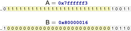
The encoder has not yet shifted the upper bits of A and B to the output, since they don’t match. Unfortunately, if we subtract A from B to determine the range of the next writeInterval, it will be too small to divide uniquely into further partitions. We’ve run out of numerical precision. The whole algorithm breaks.

To solve this problem, we must allow some bit shifting even in cases where the leading binary digits don’t match, such as in the above case. It ends up boiling down to a simple rule: As long as the second bit of A is 1 and the second bit of B is 0, keep shifting A to the output.

In doing so, we end up having to account for some funky scenarios: A becomes greater than B; we have to perform some lerps which wrap around the range of an integer; and there are cases where we need to “carry a one” back into previous bits we’ve already written to the bit stream. I won’t drill into all the details here, because it would be too boring, and I assume the handful of readers who are interested enough will study the source code anyway. In short, once everything is taken care of, range never dips below 0x40000000, providing plenty of precision.

Evidence of Memory Efficiency

I modified the source code so that it outputs some statistics to stderr, and implemented a Python function to validate the program using whatever input sequence you provide. Here’s the output from a few trial runs:

$ python -i validate.py
>>> from random import *
>>> validate([randint(0, 99999999) for i in xrange(1000000)])
Result OK after 34.537 secs
minRange=0x40000012 maxCircularBytes=1011728
>>> validate([99999999] * 1000000)
Result OK after 25.832 secs
minRange=0x40000231 maxCircularBytes=1011732
>>> validate([62 * i for i in xrange(999999)] + [99999999])
Result OK after 15.247 secs
minRange=0x40000631 maxCircularBytes=1011728
>>> validate([int(gauss(99999999, 1000000)) % 100000000 for i in xrange(1000000)])
Result OK after 29.216 secs
minRange=0x40000006 maxCircularBytes=1011728

The highlighted number tells us the maximum number of bytes in use by the circular buffer during each trial run. No matter what I tried, I couldn’t make it consume more than 1011732 bytes. That’s well within the limit of 1013000 bytes reserved for the buffer.

It’s also remarkably close to the fundamental limit of 1011717 bytes which we derived in the last post, especially considering a few bytes are wasted at the end of the sequence when flushing the BitWriter.

Pseudo-Mathematical Proof of Efficiency

It should be possible to construct a mathematical proof giving an upper bound on the amount of memory needed to encode a sorted sequence using this method. I’m totally going to handwave through this part, but if you accept that the encoding process works the same even if you “break up large deltas” using a lookup table of just 2 elements, 0 and D, it follows that it takes

to output a single value in the sorted sequence, which happens 1000000 times, and

to increment the value by 1, which happens at most 99999999 times. Therefore, in pure theory, it shouldn’t take more than 6.65821147 × 1000000 + .01435529 × 99999999 ≈ 8093740 bits to encode any sequence, which is pretty close to the fundamental limit we derived earlier. The proof would also have to add some small epsilon value to account for the loss of precision that happens at each step using fixed-point math, but I haven’t figured that out, and I’m not really interested in going that far.

In wrapping up this subject, I learned something interesting while reading up on arithmetic coding. Dozens of US patents related to the technique have been granted in recent years. One side effect from these patents is that, apparently, most JPEG images in use today take up to 25% more space than they would without the existence of such patents. It’s rather funny (and a bit sad) when you consider that the intended goal of the patent system is to advance science and technology.